Recording

Homework submission
Submitting all three homework assignments will qualify you for a free Professional Training (value of 500€), a certificate of participation and will give you a chance to win a fully-working prototype of a 3D printer with your design modifications.
Homework 2 - Deadline 27.06 4:00pm
Please use the form to submit your homework
Exercise
Our aim is to investigate the mechanical behaviour of the frame of the 3D printer. We will therefore run two different simulations. First of all, we have to identify the critical eigenfrequencies of the printer frame. Later on, this information will be used as an input to analyze the physical response of our system.
Step-by-Step Instructions
NOTE: This tutorial was updated on 10/2016 to match the updated version of the platform
Meshing
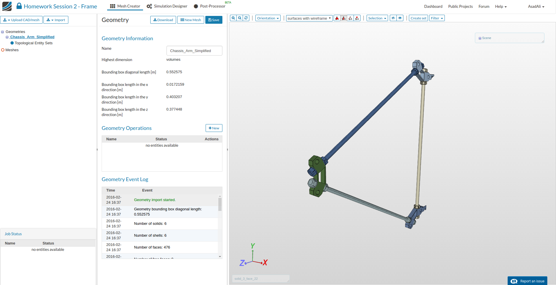
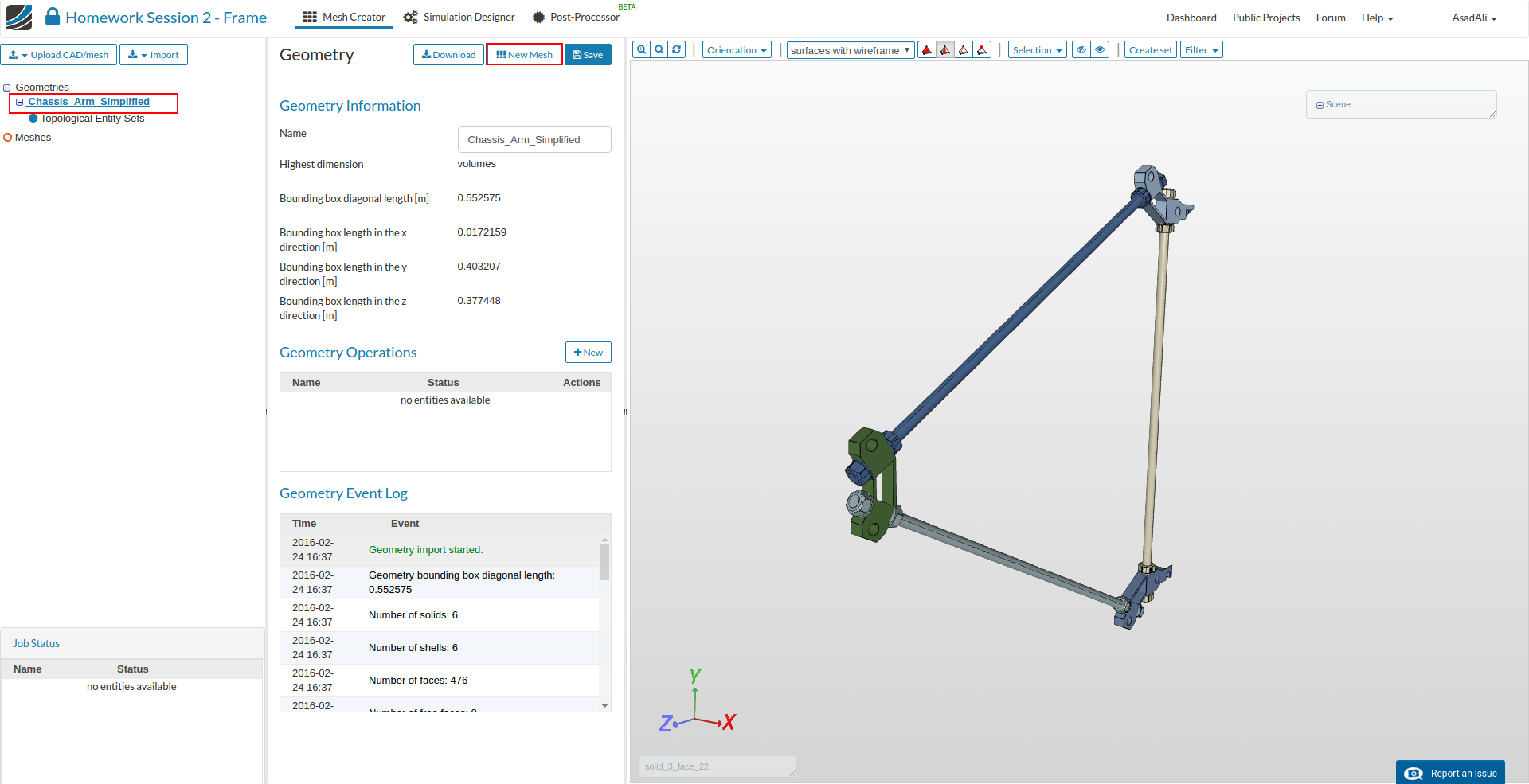
First of all you have to import the geometry into your SimScale workspace. For this, you only have to click on this link. Please note that this can take several minutes.
To make this project public, edit the project properties
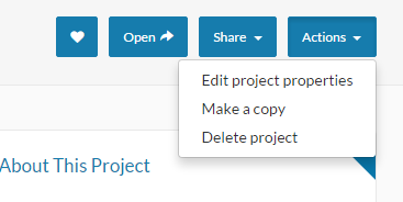
and change the visibility to public

Now select the geometry and click on the New Mesh from the middle column to add start a new mesh setup for this geometry.
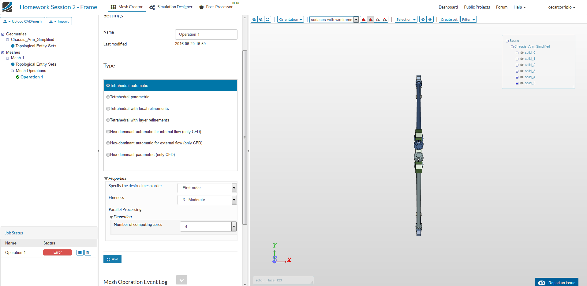
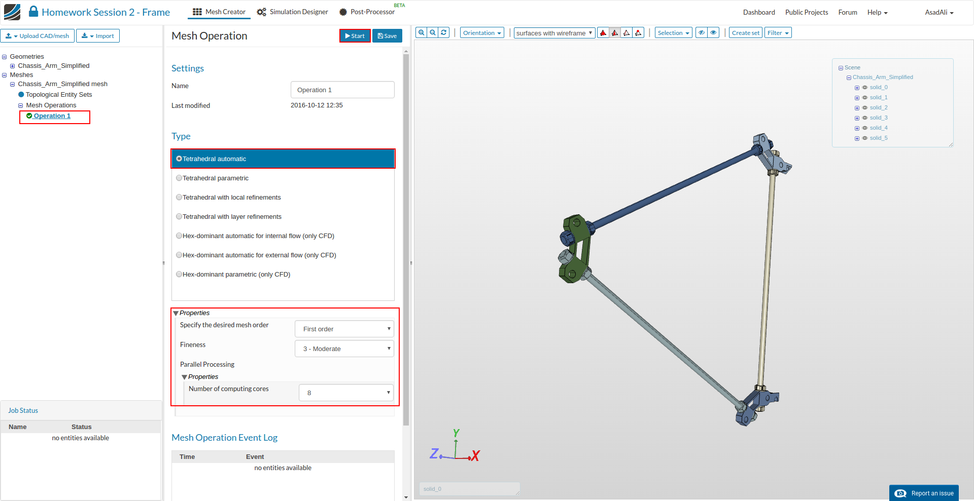
A new mesh tree will be added in the left column and in the middle column you can select the mesh type and other parameters. Select Tetrahedral automatic from the list and choose the following settings
- Specify the desired mesh order: First order
- Fineness: 3 - Moderate
- Number of computing cores: 8
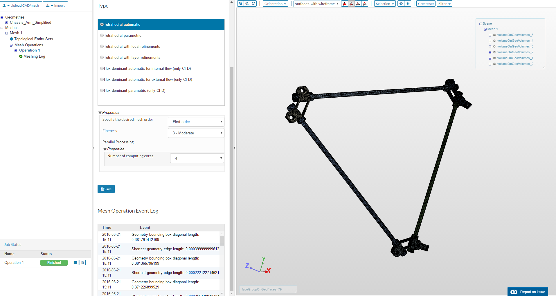
Once done press Start button to start the mesh.
Simulation Setup I
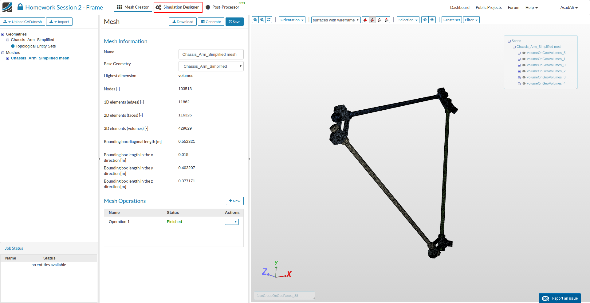
Please switch to the Simulation Designer by clicking the related button in the main ribbon bar
Click on the New button to create a simulation run.
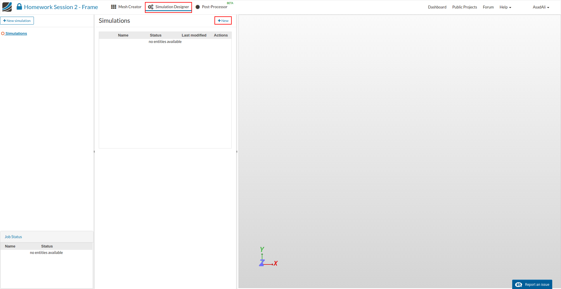
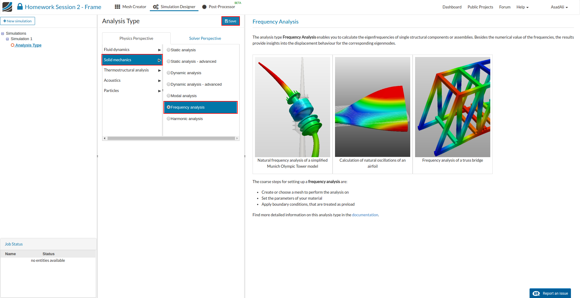
This will open an additional column in the middle. Here you can select which kind of simulation you want to run. In our case we will run a Frequency analysis to receive critical frequencies for the harmonic analysis.
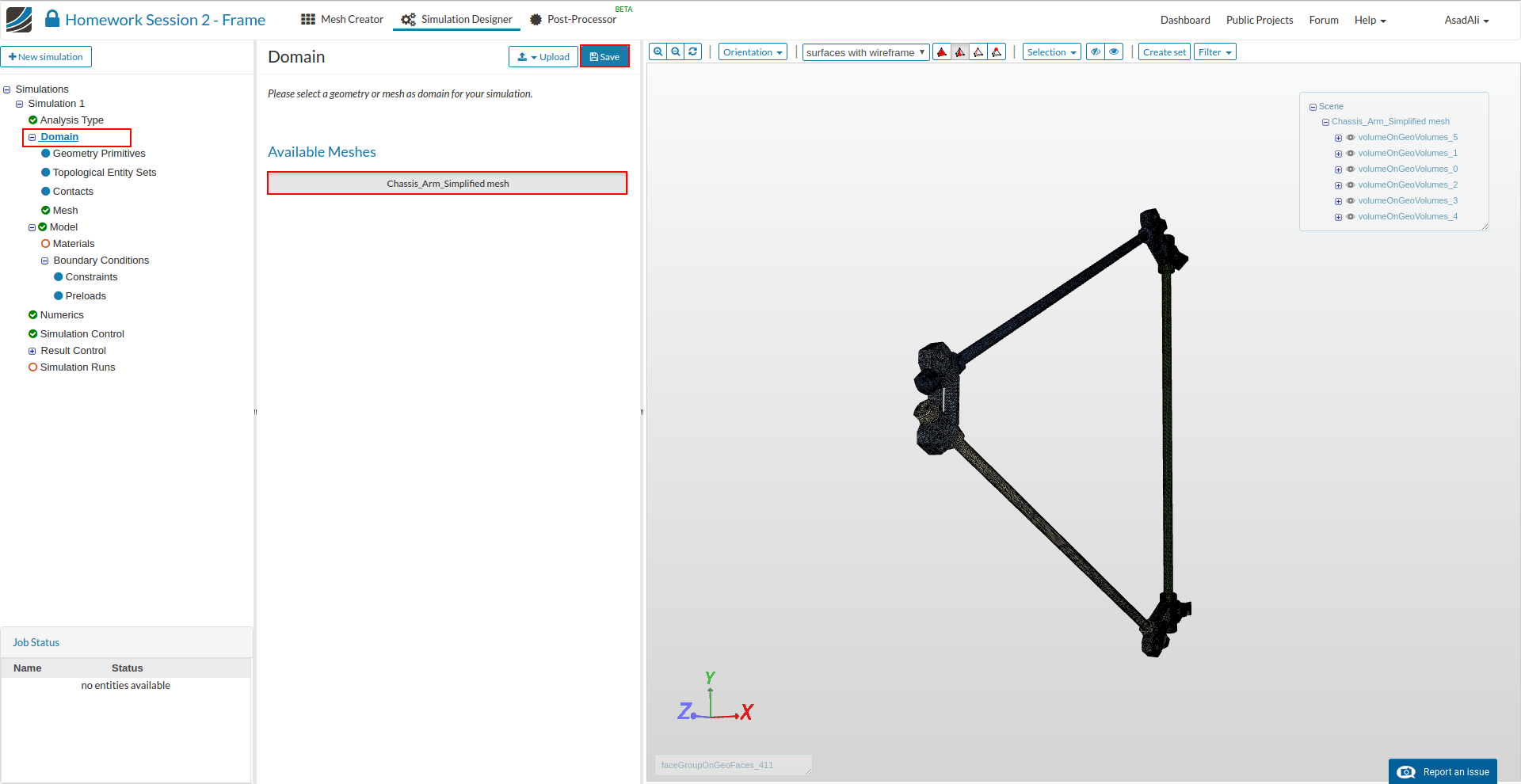
Next you have to specify which mesh you want to use for your simulation. Click on the Domain item in the project tree and select the respective mesh from the menu which appears in the middle column. Don’t forget to save your selection.
Since we are simulating an assembly of parts it is necessary to define the interactions withing the assembly and with its environment. We will therefore define this so called Contacts, which are also covering the physical interaction between parts. This topic was also covered very detailed during the last webinar. You can find the section about contacts here
Without the contacts, the solver does not knows which parts are connected to each other. To define the full interactions between the six different solids we need at least nine contacs.
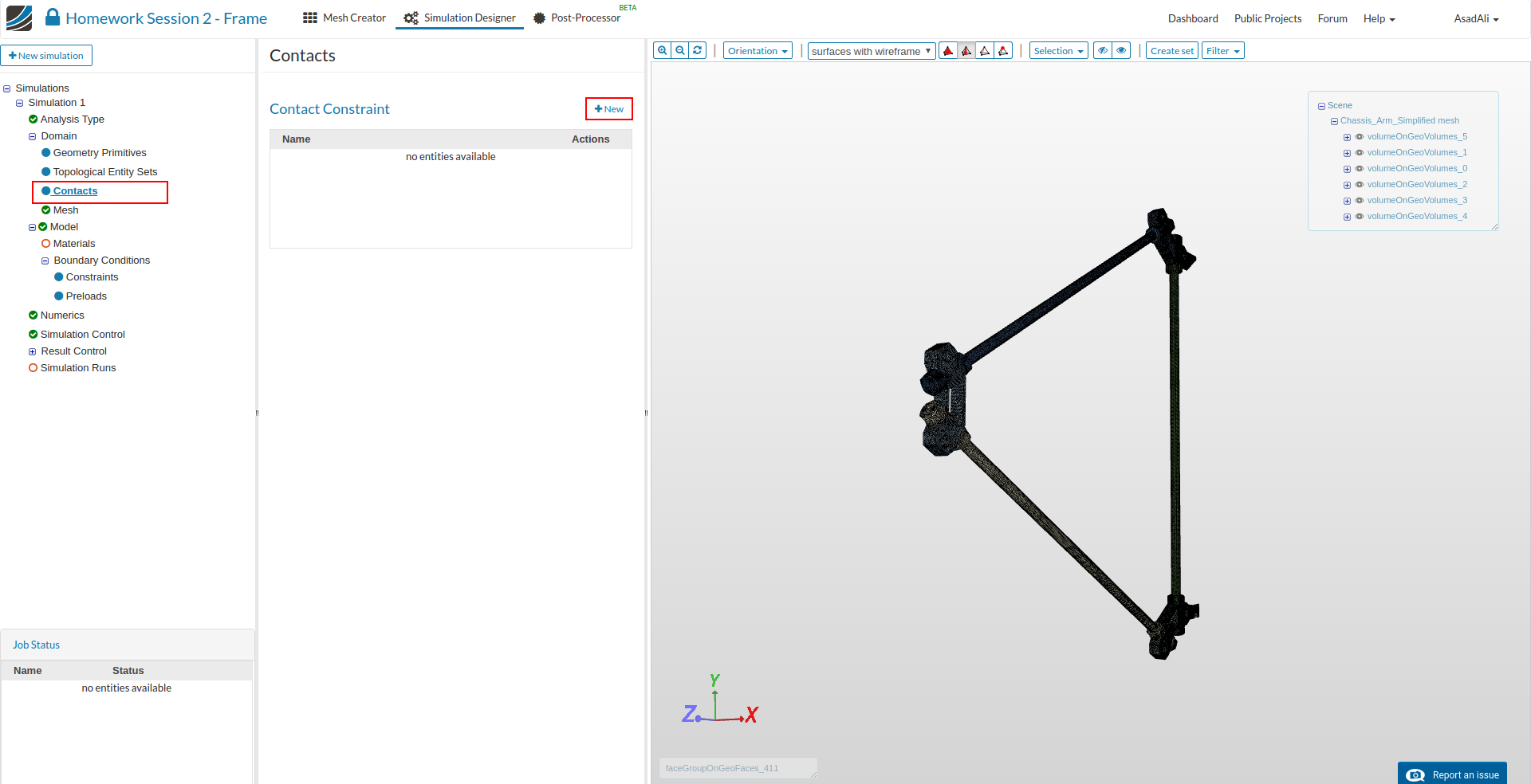
Please click on the Contacts sub-item in the project tree. This will open a new middle column windows where you can manage existing and create new contacts. Next, click on the New button
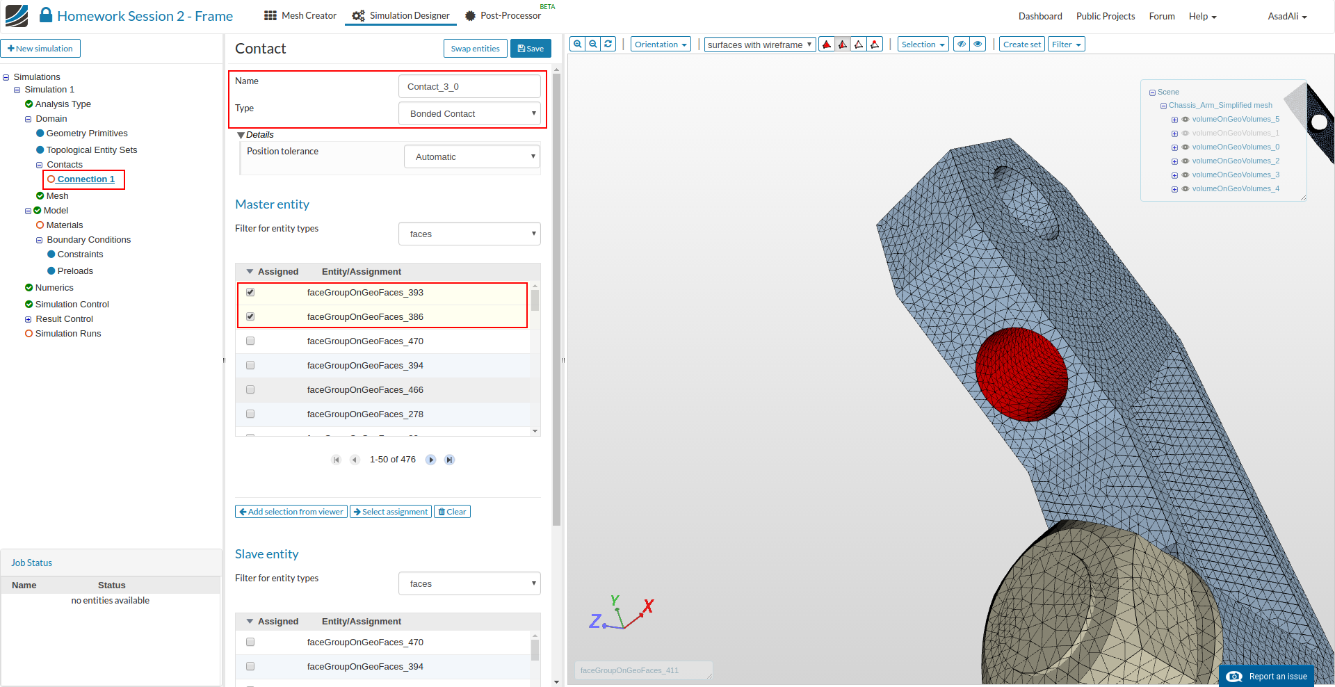
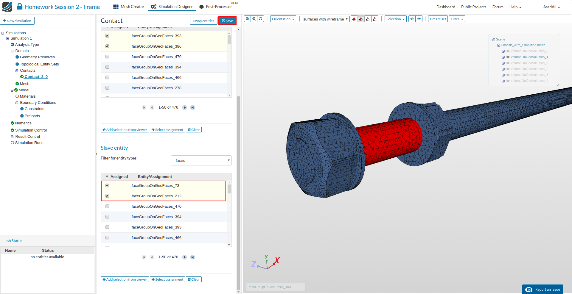
Contact #1 - Connector (solid_3) and Rod (solid_1)
This contact is necessary to connect the Connector (solid_3) and Rod (solid_1)
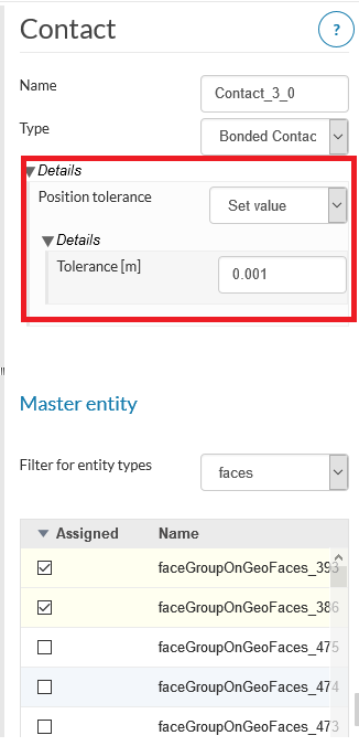
- Name: Contact_3_0
- Type: Bonded Contact
- Master entity: faceGroupOnGeoFaces_393 (volumeOnGeoVolumes3), faceGroupOnGeoFaces_386 (volumeOnGeoVolumes3)
- Slave entity: faceGroupOnGeoFaces_73 (volumeOnGeoVolumes1), faceGroupOnGeoFaces_212 (volumeOnGeoVolumes1)
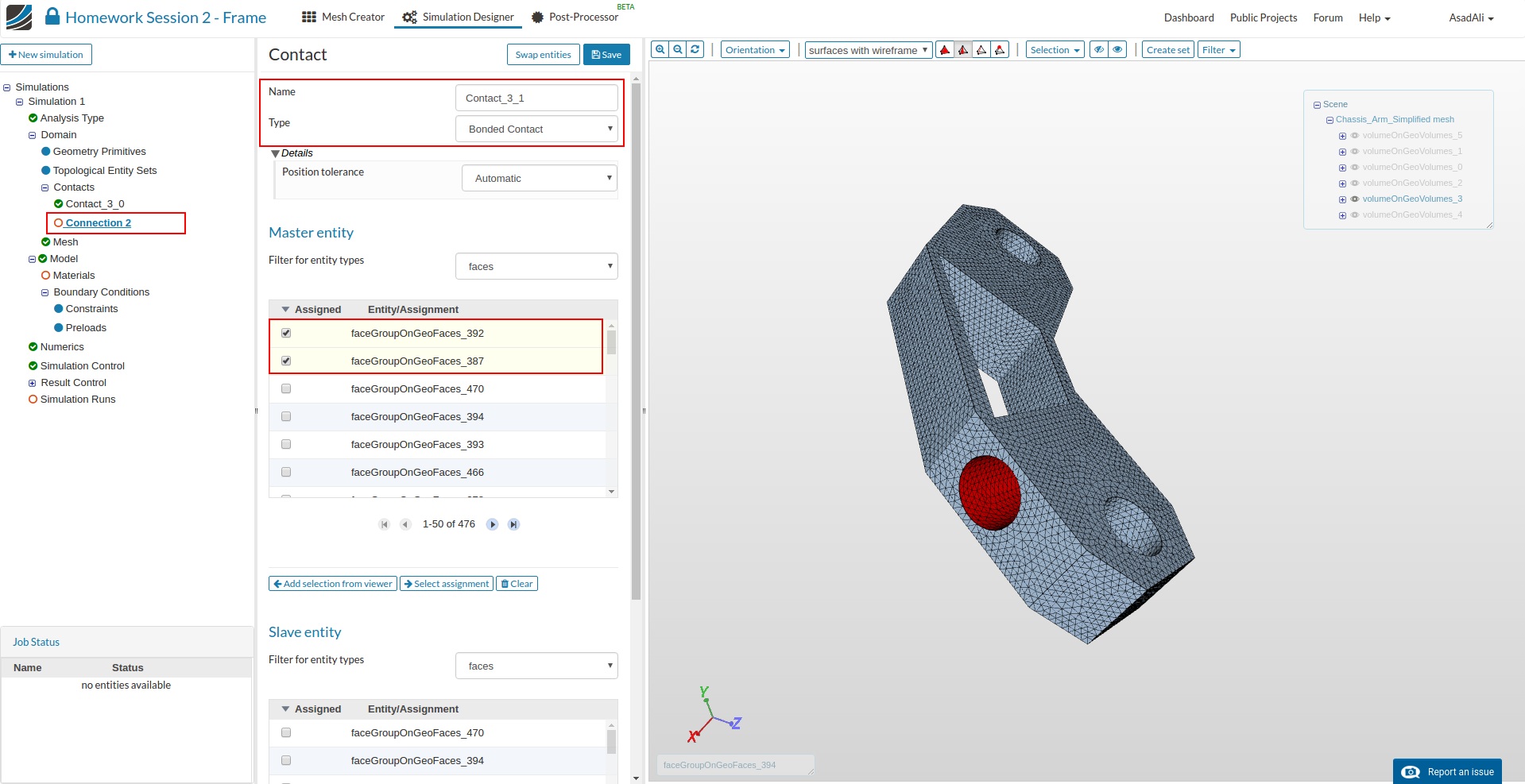
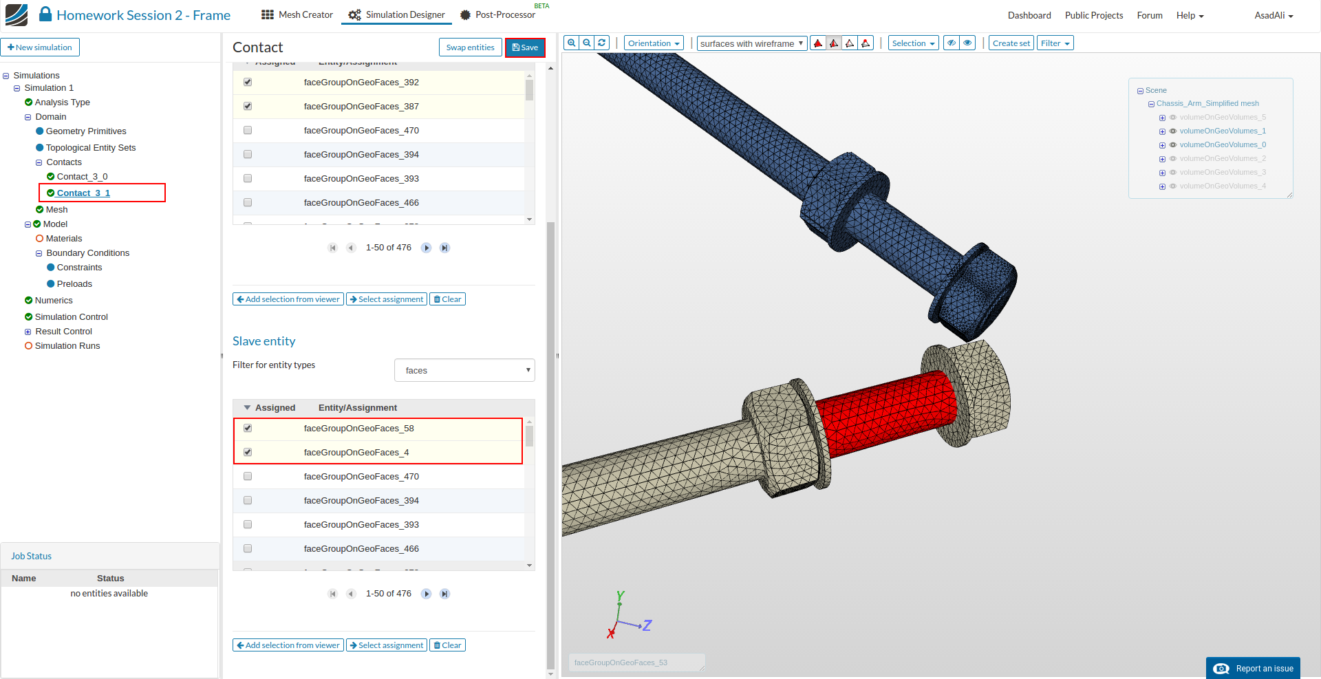
Contact #2 - Connector (solid_3) and Rod (solid_0)
This contact is necessary to connect the Connector (solid_3) and Rod (solid_0)
- Name: Contact_3_1
- Type: Bonded Contact
- Master entity: faceGroupOnGeoFaces_392 (volumeOnGeoVolumes3), faceGroupOnGeoFaces_387 (volumeOnGeoVolumes3)
- Slave entity: faceGroupOnGeoFaces_4 (volumeOnGeoVolumes0), faceGroupOnGeoFaces_58(volumeOnGeoVolumes0)
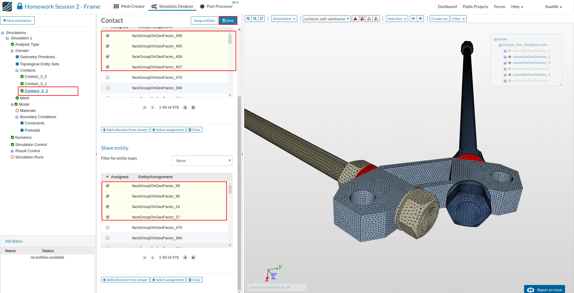
Contact #3 - Connector (solid_3) and both Rods (solid_0 and solid_1)
This contact is necessary to connect the Connector (solid_3) and Rod (solid_1)
- Name: Contact_3_2
- Type: Bonded Contact
- Master entity: faceGroupOnGeoFaces_405 (volumeOnGeoVolumes3), faceGroupOnGeoFaces_406 (volumeOnGeoVolumes3), faceGroupOnGeoFaces_407 (volumeOnGeoVolumes3), faceGroupOnGeoFaces_408 (volumeOnGeoVolumes3)
- Slave entity: faceGroupOnGeoFaces_96 (volumeOnGeoVolumes1), faceGroupOnGeoFaces_99(volumeOnGeoVolumes1), faceGroupOnGeoFaces_24 (volumeOnGeoVolumes0), faceGroupOnGeoFaces_27 (volumeOnGeoVolumes0)
Please find below and overview for the missing contacts and create them:

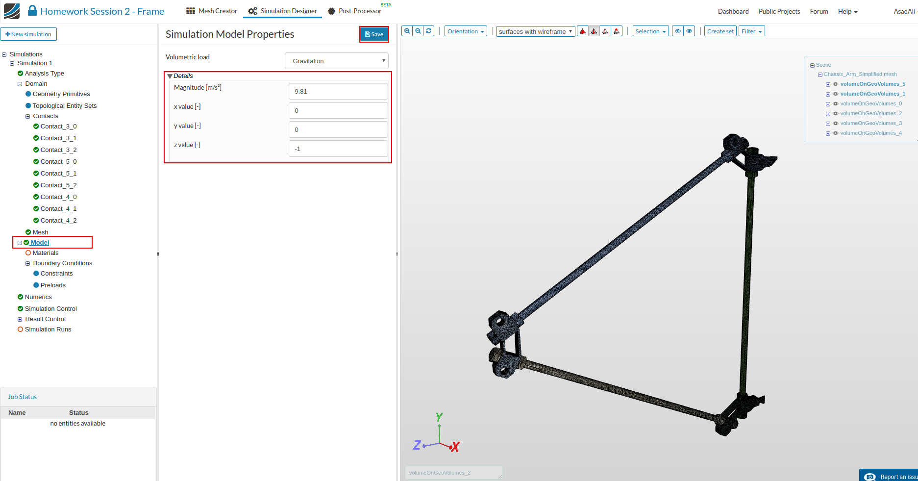
Next we have to define the physical Model we want to use for this simulation. Click therefore on the Model item in the project tree which will open a middle column windows. Here you can define the gravitation.
- Magnitude: 9.81
- x value: 0
- y value: 0
- z value: -1
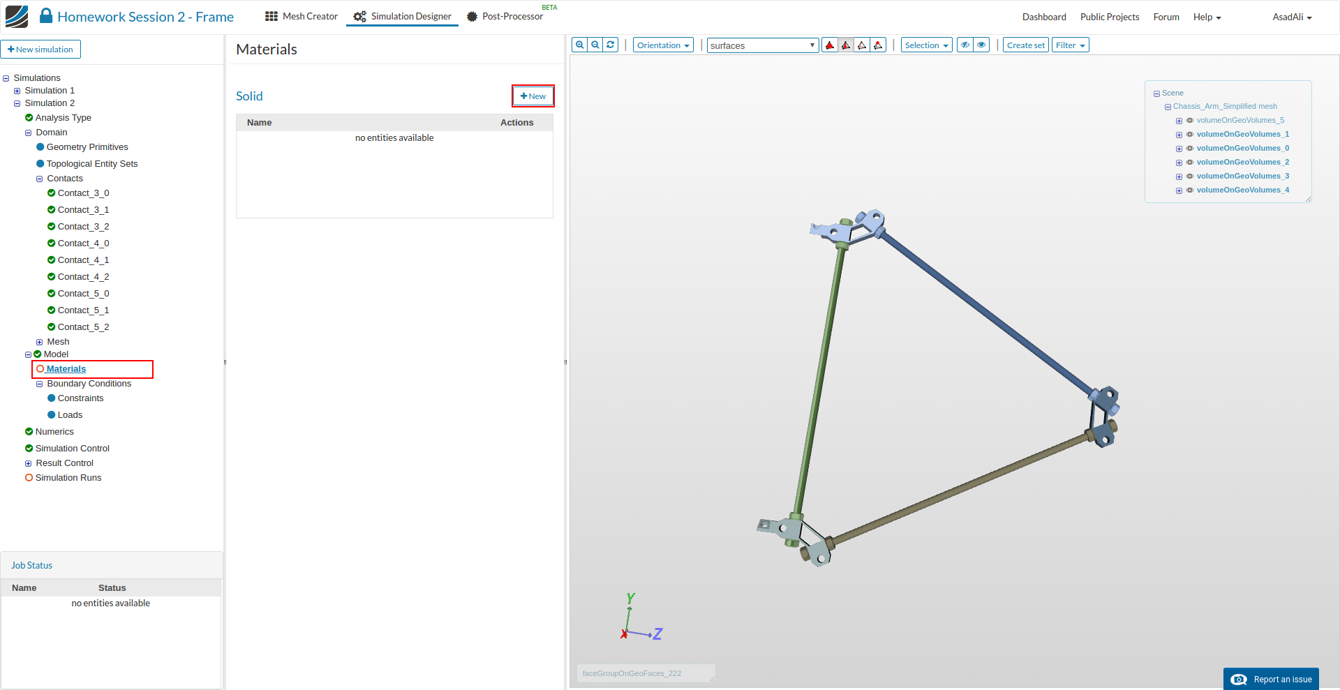
Now we define and assign material properties to the different parts. Click on the** Materials** in the project tree. This will open a middle column menu where you can edit and create materials and assign them to volumes. Click on the New button.
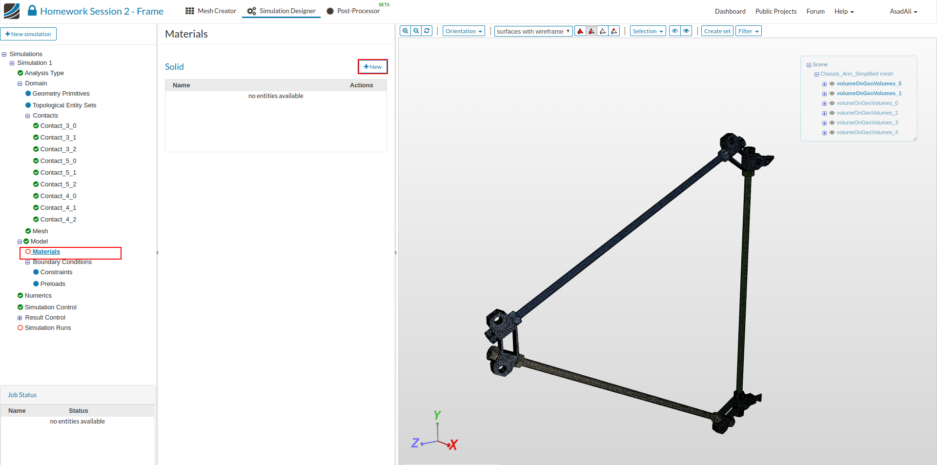
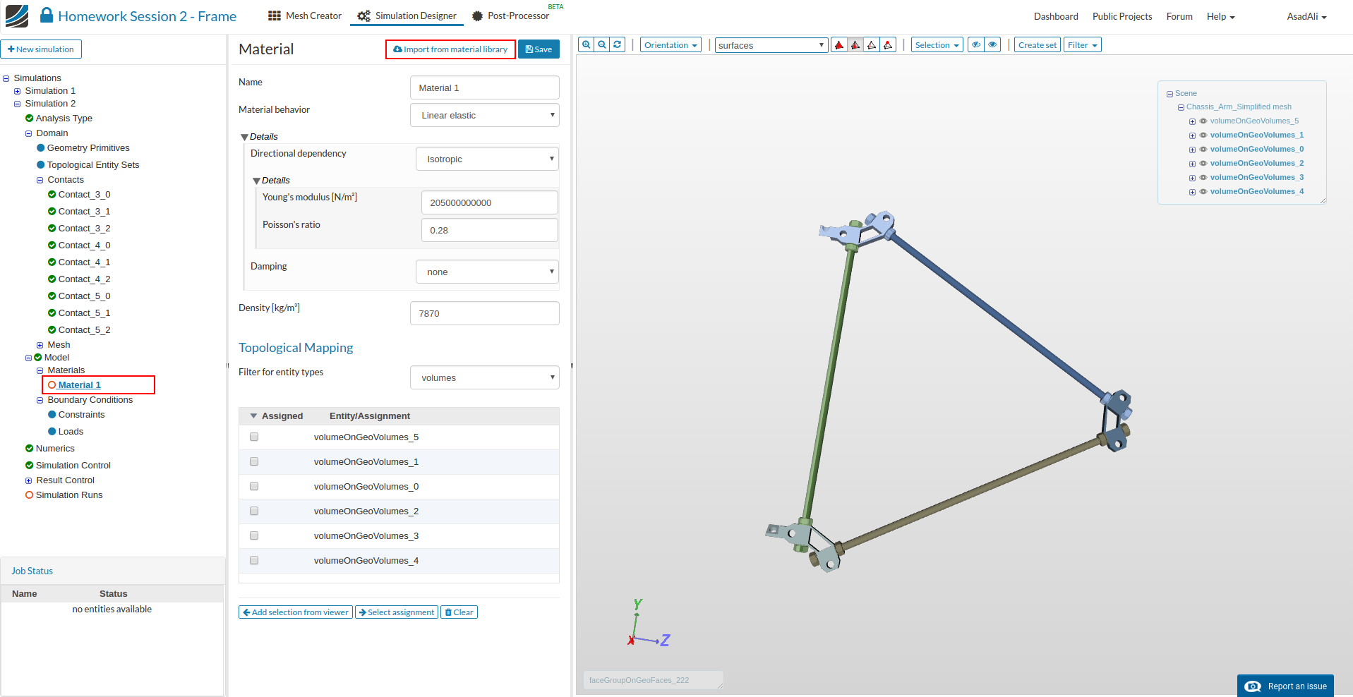
Now you can define your new material based on your own material proporties or access our Material Library which includes ready-to-use material models for several materials.
Next we will assign the steel material model to the screws and the engine. Add an additional material to your project tree.
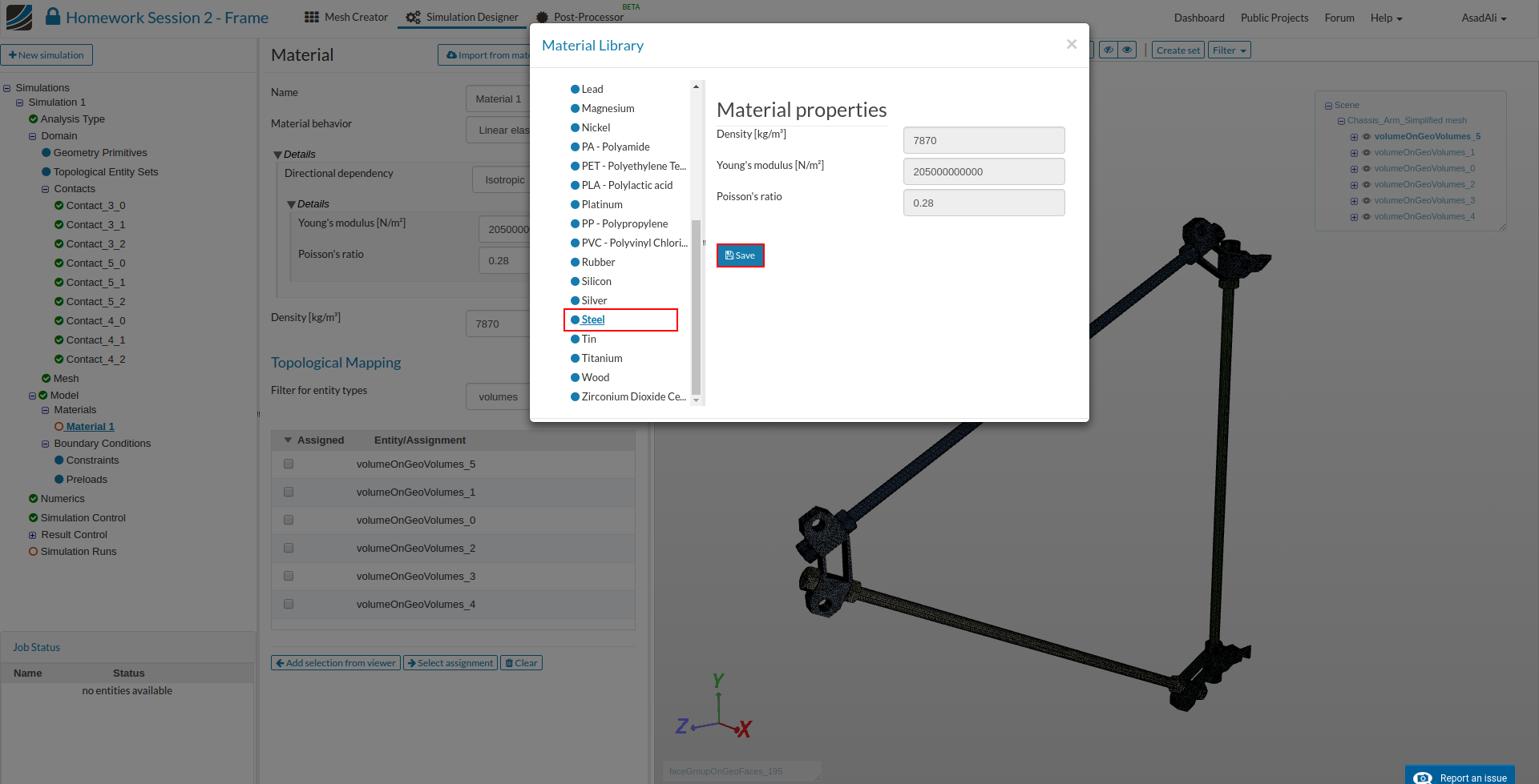
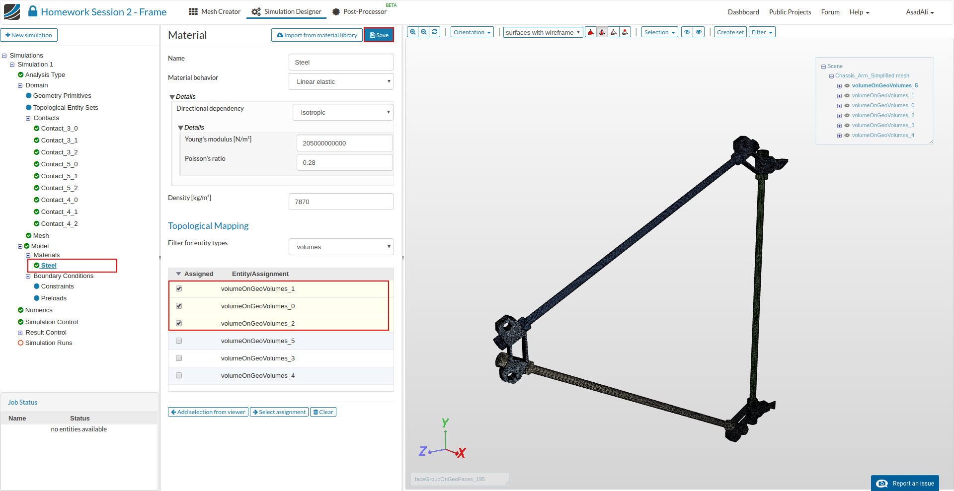
Now we will access our material library instead of creating the material model manually. Click on the Import from material library which will open a widget.
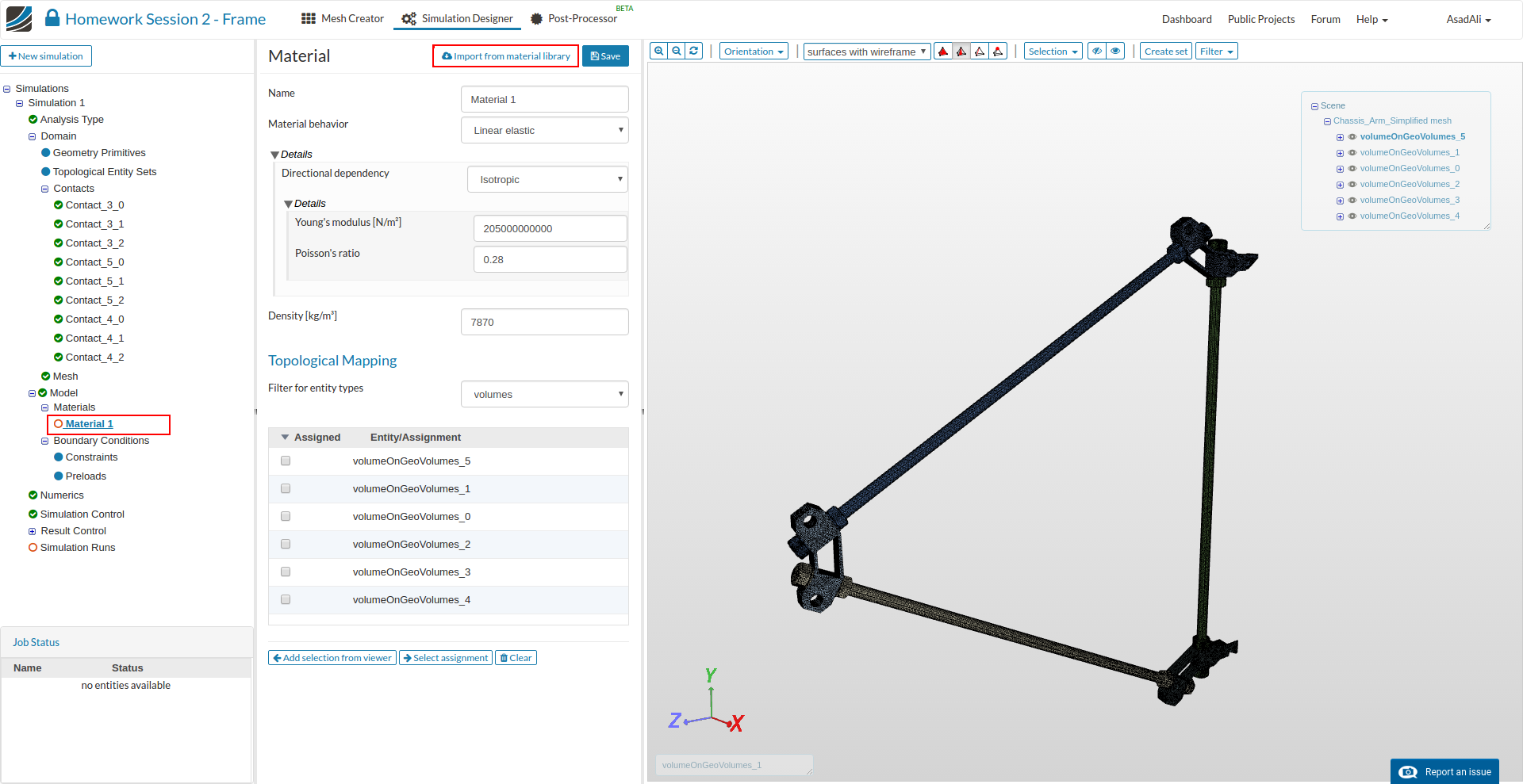
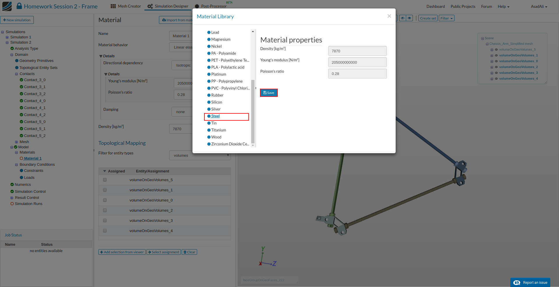
Please select steel from the list on the left side and save your selection by clicking the related button.
Now assign the material to the rods (volumeOnGeoVolumes_0, volumeOnGeoVolumes_1, volumeOnGeoVolumes_2).
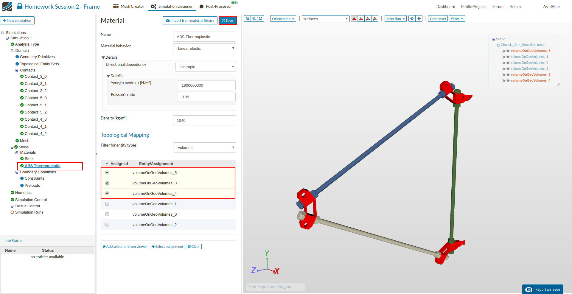
Please add a new material with following settings. Instead of using the library we have to define the material manually:
- Name: ABS Thermoplastic
- Young’s Modul: 1800000000
- Poisson’s ratio: 0.35
- Densiy: 1040
And assign it to the connectors (volumeOnGeoVolumes_3, volumeOnGeoVolumes_4, volumeOnGeoVolumes_5)
Next we can start to define the boundary conditions. Click on the Boundary Conditions item in the project tree.
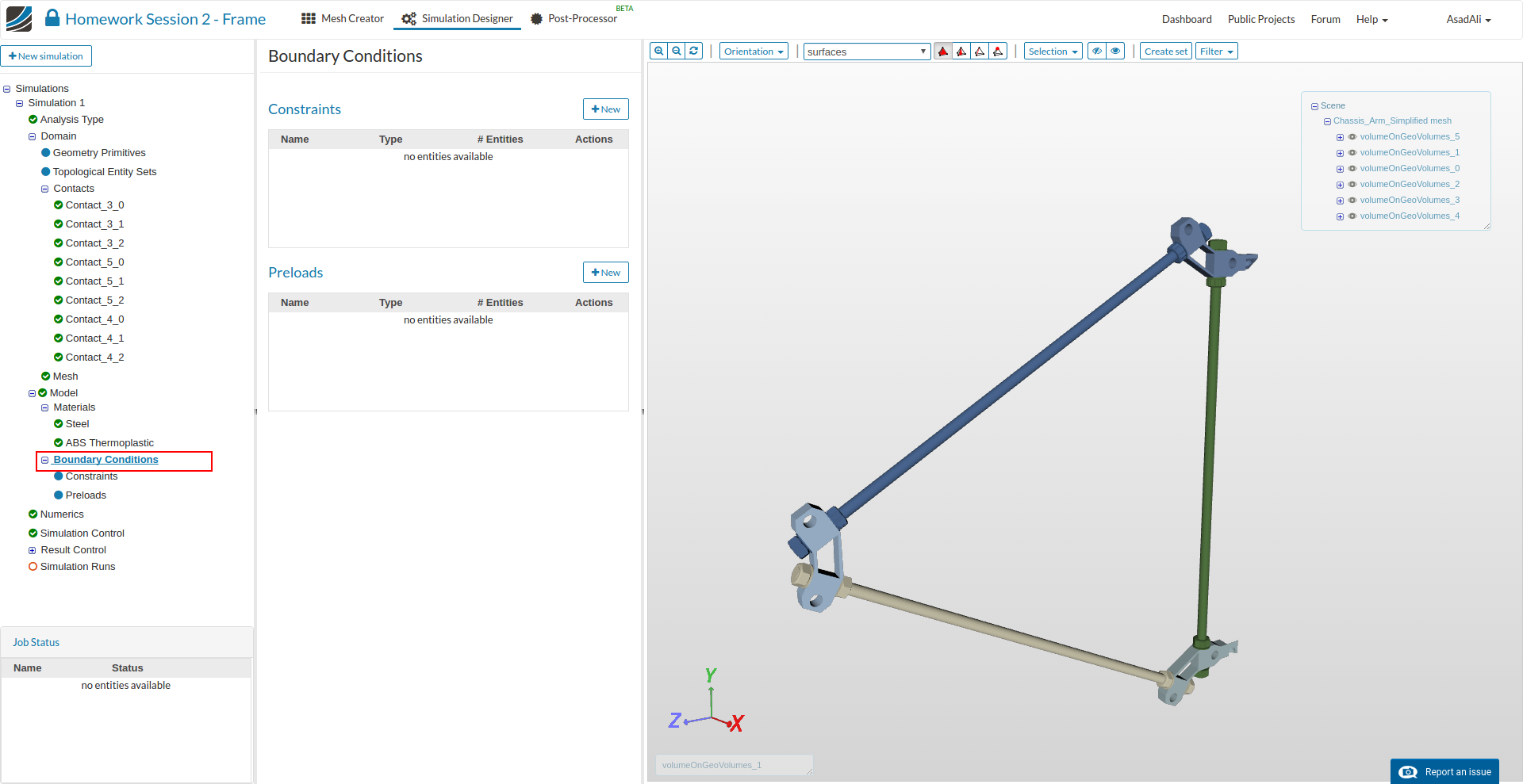
There are two kinds of boundary conditions for structural simulations.
Constraint conditions are used to limit the degrees of freedom of the model. Load conditions are applying an external load to the model
Due the fact that this is only a frequency analysis we only need to define two contraint boundary conditions (external loads are not important at this stage).
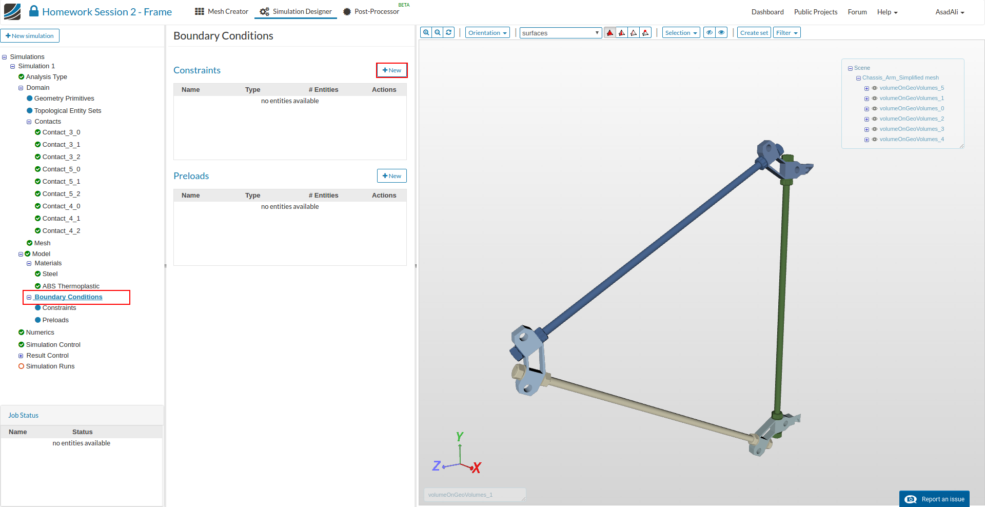
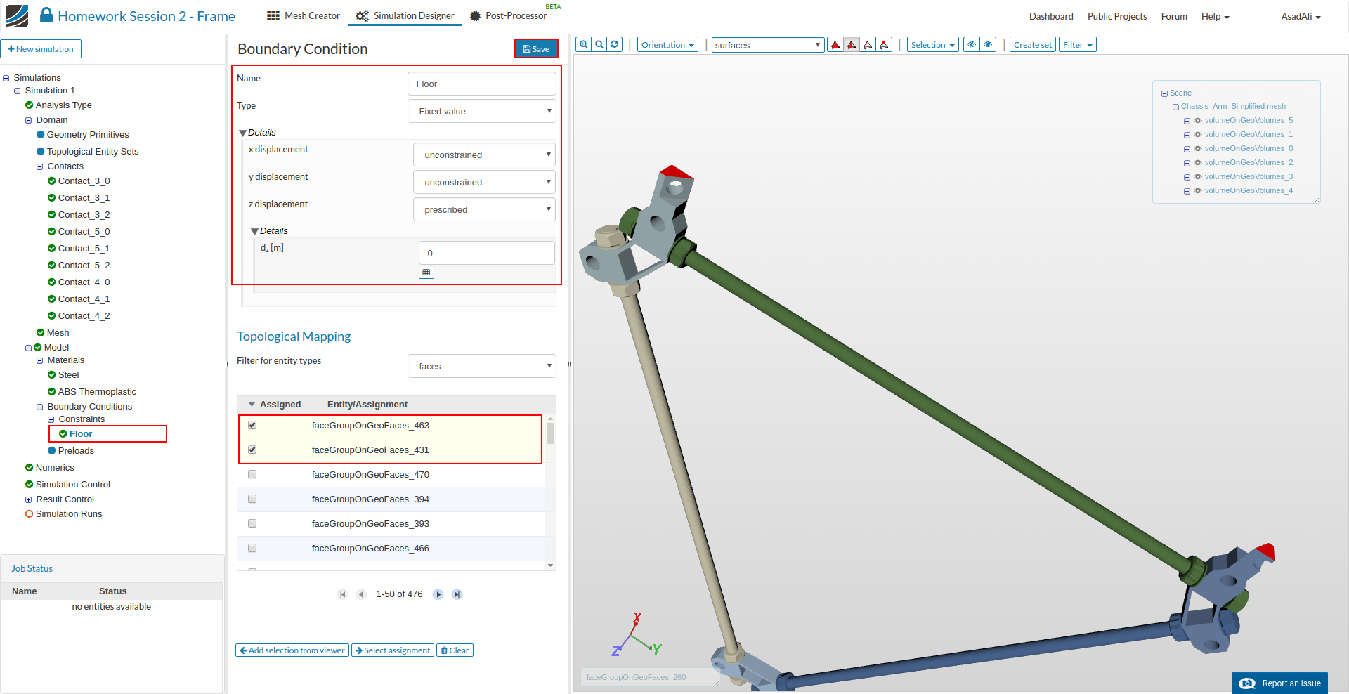
Floor
This boundary condition is necessary since the printer is standing on a table and can not move up or down
- Name: Symmetry XY-planeType:
- Fixed Value
- x displacement: unconstrained
- y displacement: unconstrained
- z displacement: prescribed with a value of 0
And assign it to faceGroupOnGeoFaces_463 (volumeOnGeoVolumes_5) and faceGrouponGeoFaces_431 (volumeOnGeoVolumes_4)
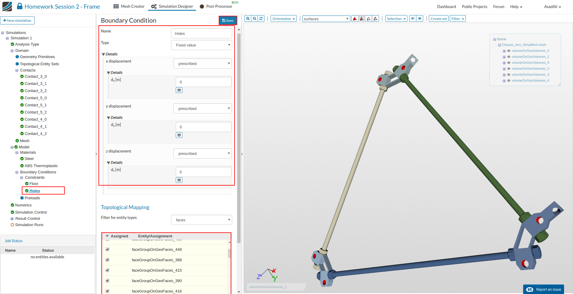
Holes
This boundary conditions is necessary to consider the fact that the frame section we are simulating is connected to other parts.
- Name: Holes
- Fixed Value
- x displacement: prescribed with a value of 0
- y displacement: prescribed with a value of 0
- z displacement: prescribed with a value of 0
And assign it to faceGroupOnGeoFaces_450, faceGroupOnGeoFaces_449, faceGroupOnGeoFaces_448, faceGroupOnGeoFaces_447, faceGroupOnGeoFaces_418, faceGroupOnGeoFaces_417, faceGroupOnGeoFaces_416, faceGroupOnGeoFaces_415, faceGroupOnGeoFaces_391, faceGroupOnGeoFaces_390, faceGroupOnGeoFaces_389, faceGroupOnGeoFaces_388
Numerics, which is the next item in the project tree, can be skipped since the default settings are fine.
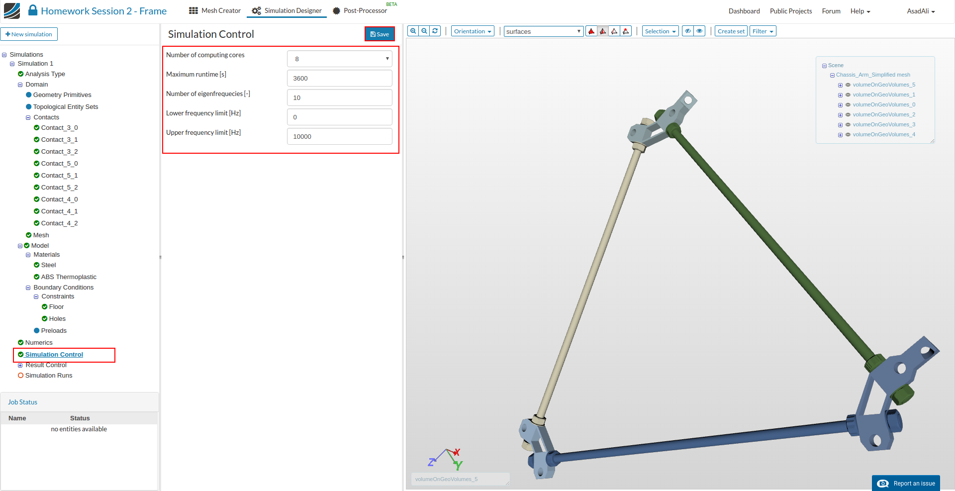
Click on the Simulation Control item in the project tree to specify how fast and accurate you want the simulation to be computed.
- Numer of Computing cores: 4
- Maximum runtime: 3600
- Number of eigenfrequecies: 10
- Lower frequency limit [Hz]: 0
- Upper frequency limit [Hz]: 10000
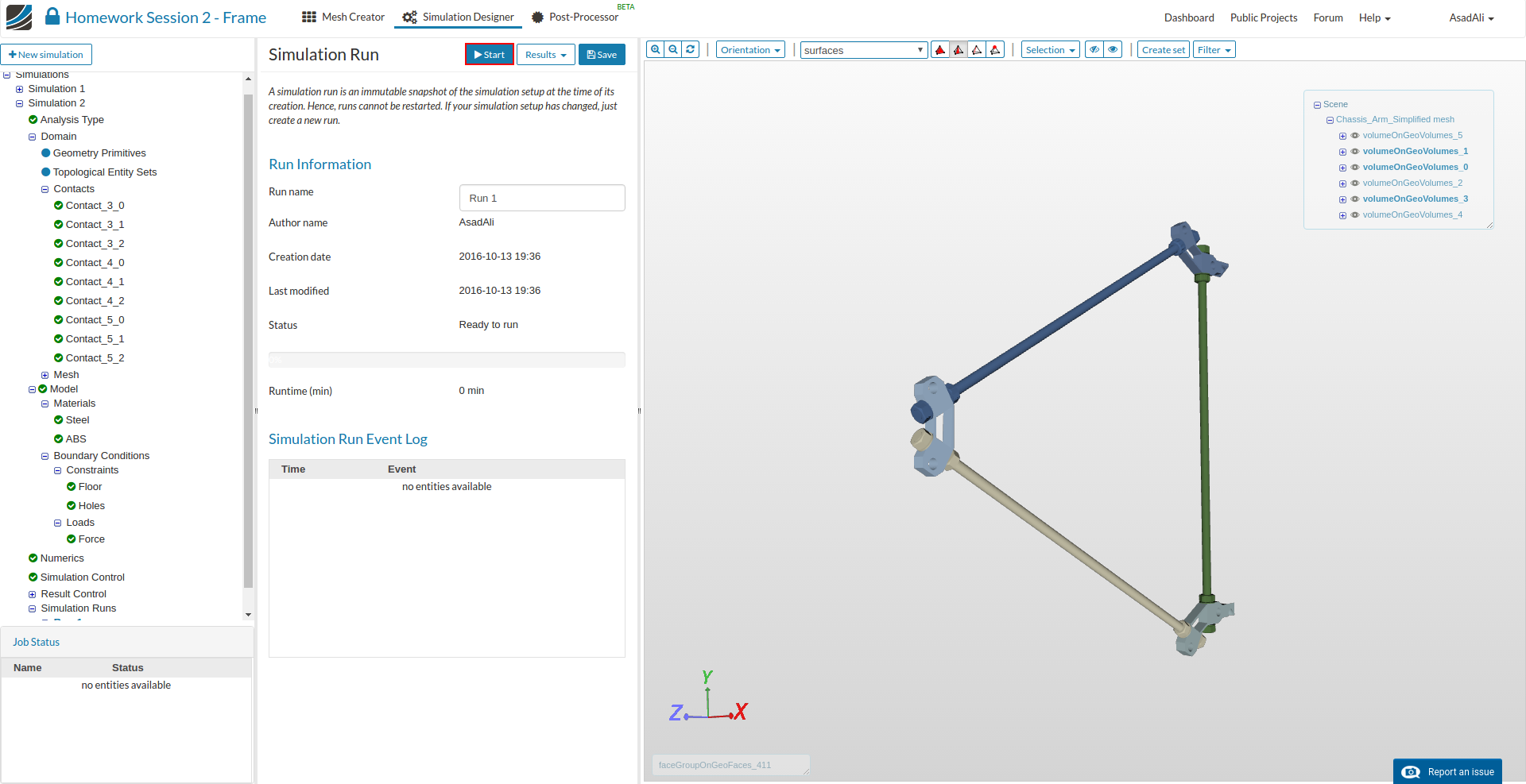
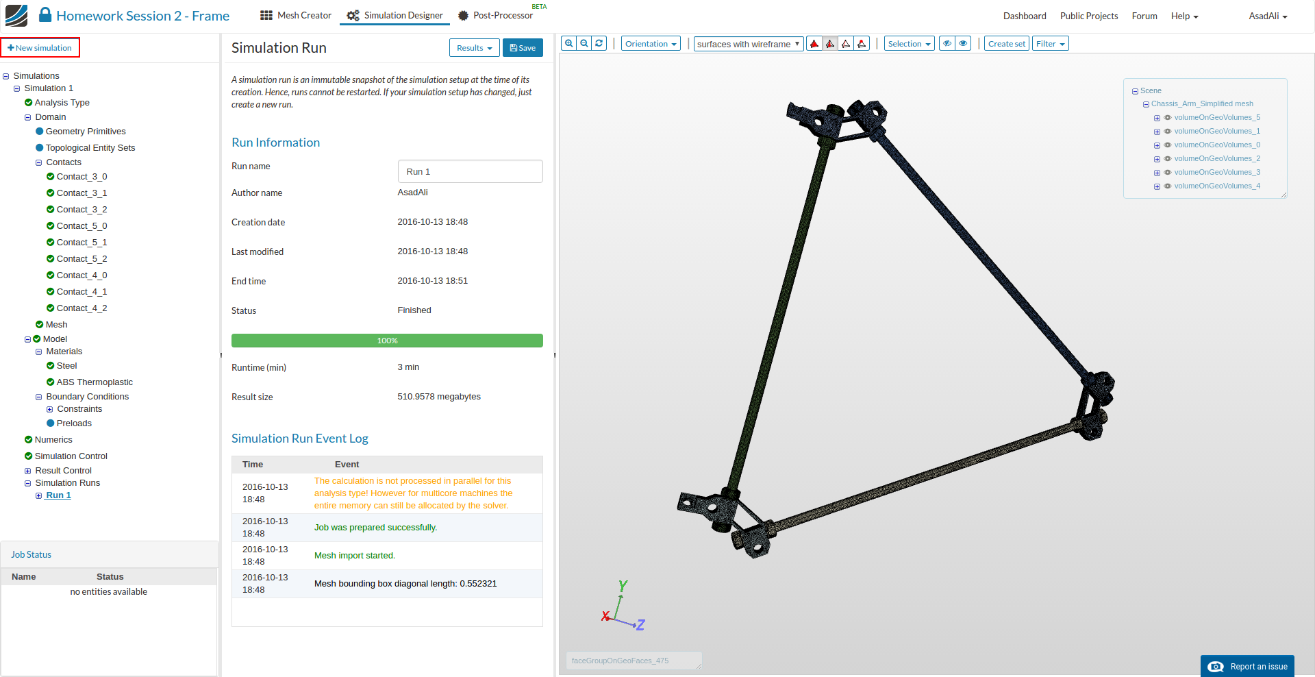
To start the simulation, click on the Simulation Run item in the tree and click on the create new run by pressing New button. This will create a snapshot of your simulation settings as a new sub-item.
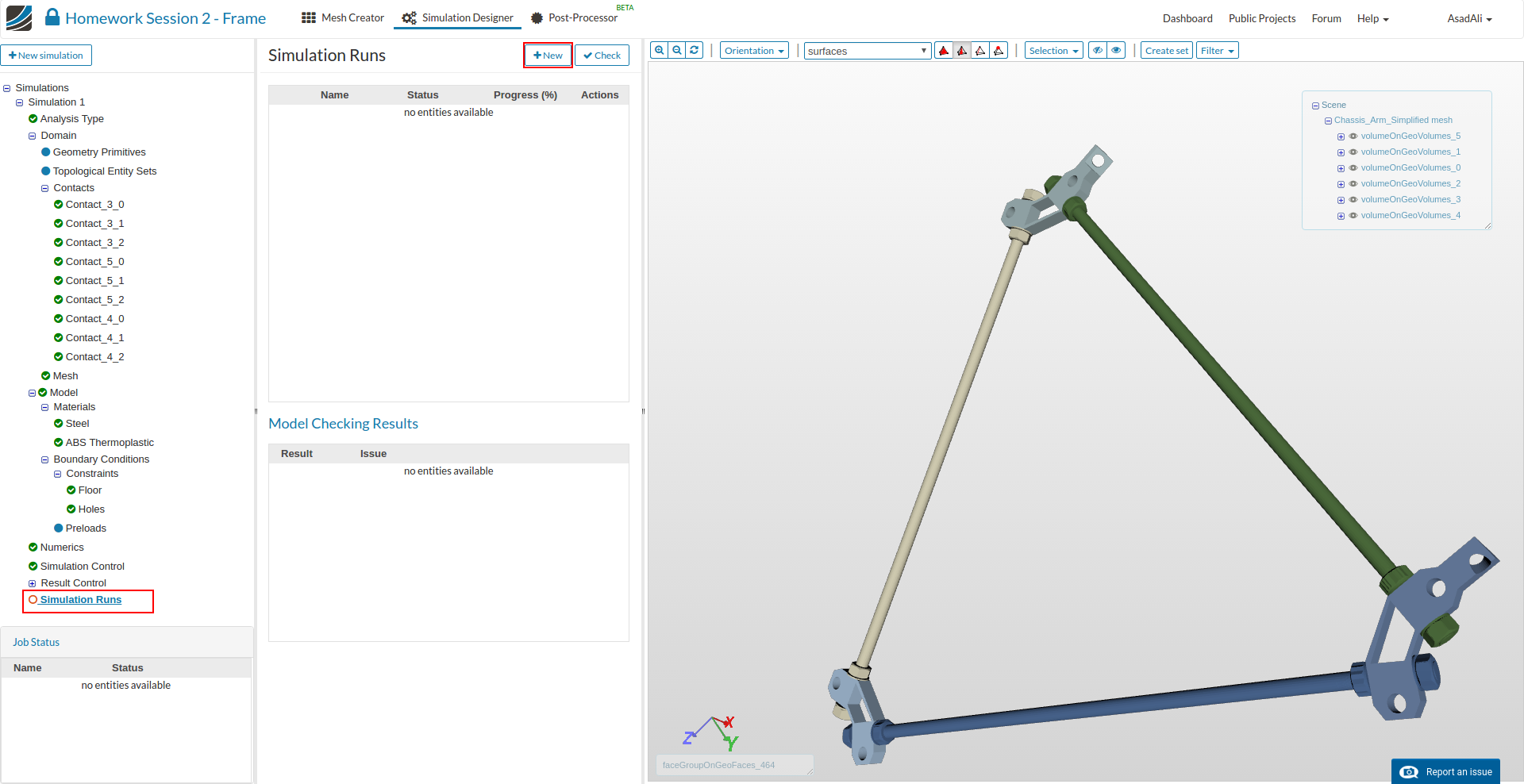
And start the simulation run by clicking the related button.
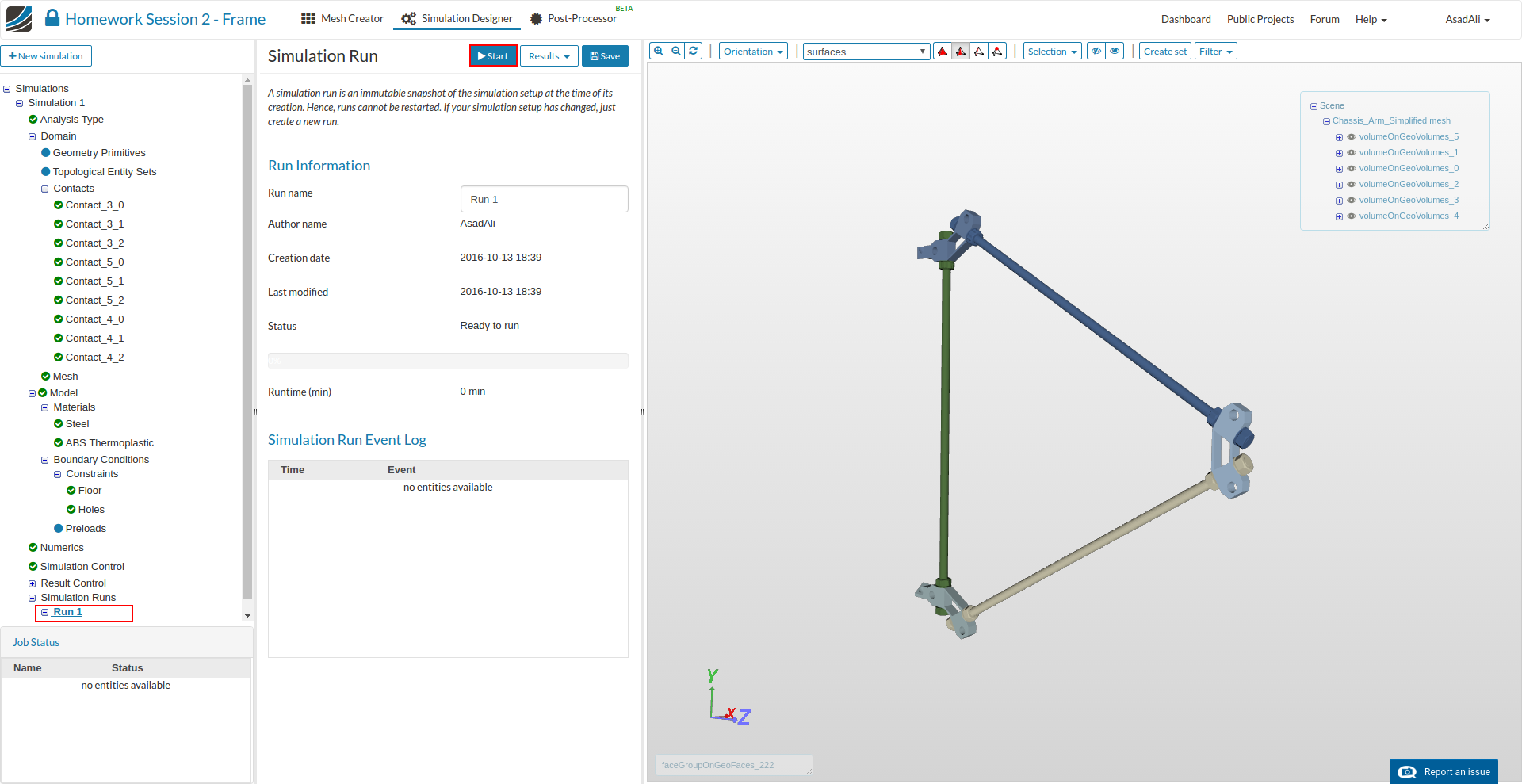
When will be notified once the simulation run is finished.
Post Processing I
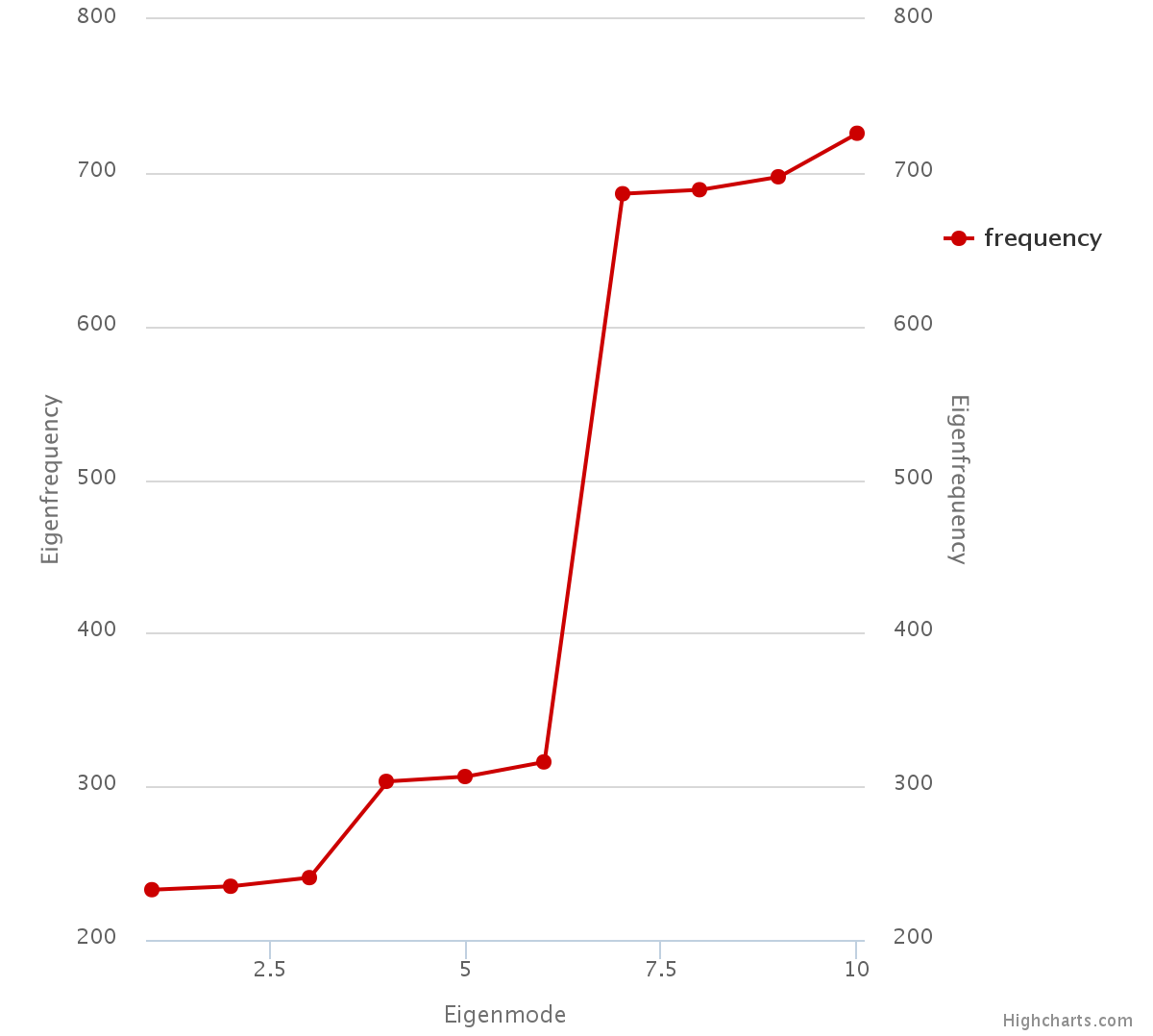
Now we will take a look at the results of our simulation. Since we are interested to find out the eigenfrequencies of the drone we will not perform a 3D post processing.
Please click on the Eigenfrequency plot sub-item in the project tree. This will open a graph which shows the first 10 eigenmodes and the related eigenfrequency.
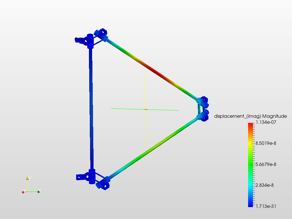
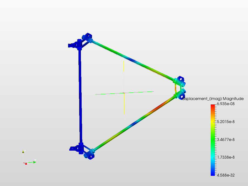
Simulation Setup II
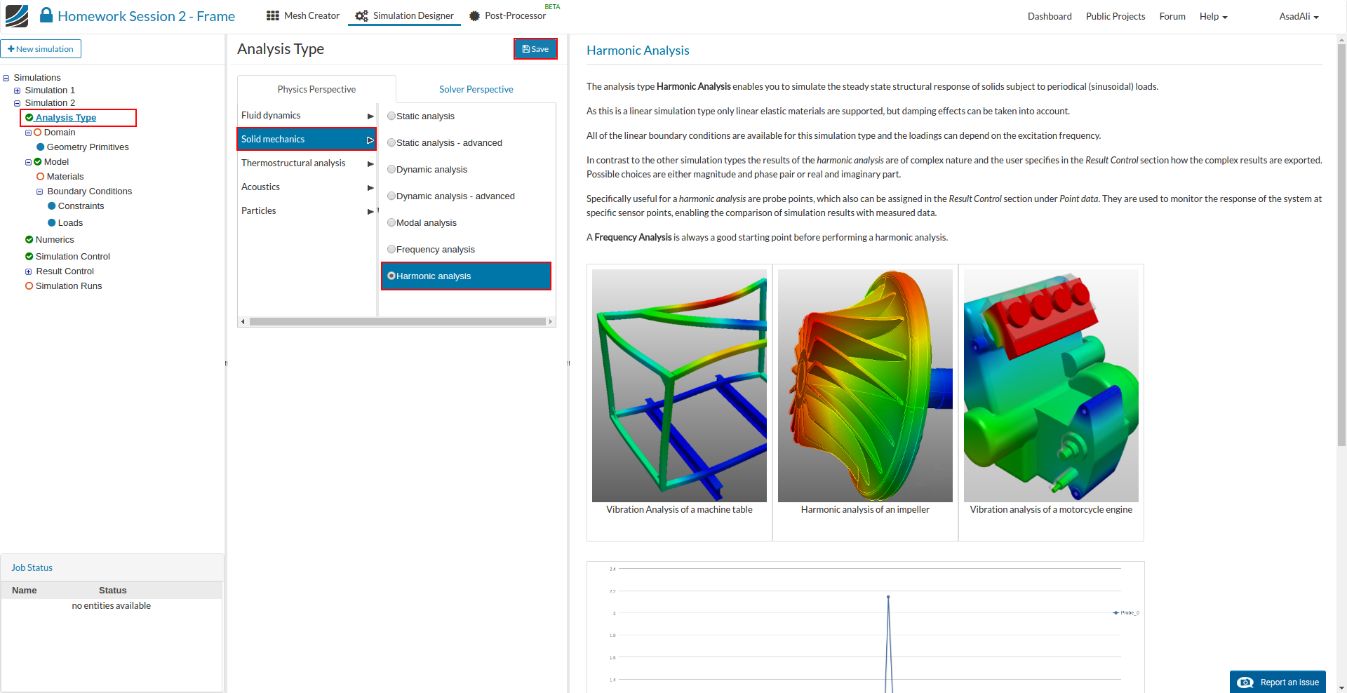
We will now create a harmonic analysis to investigate the physical response of our system.
Click on the New simulation button to create a simulation run. This will open an additional column in the middle. Here you can select which kind of simulation you want to run.
In our case we will run a Harmonic Analysis.
The next steps of the setup is equal to the Frequency Analysis of the previous section. Please assign the same mesh and create again nine contacts. **Note: Regarding the contacts you have to set the position tolerance manually (0.001m), since there is no automatic position tolerance available for this analysis type.
Now we define and assign material properties to the different parts. Click on the** Materials** in the project tree. This will open a middle column menu where you can edit and create materials and assign them to volumes. Click on the New button.
Now you can define your new material based on your own material proporties or access our Material Library which includes ready-to-use material models for several materials.
Next we will assign the steel material model to the screws and the engine. Add an additional material to your project tree.
Now we will access our material library instead of creating the material model manually. Click on the Import from material library which will open a widget.
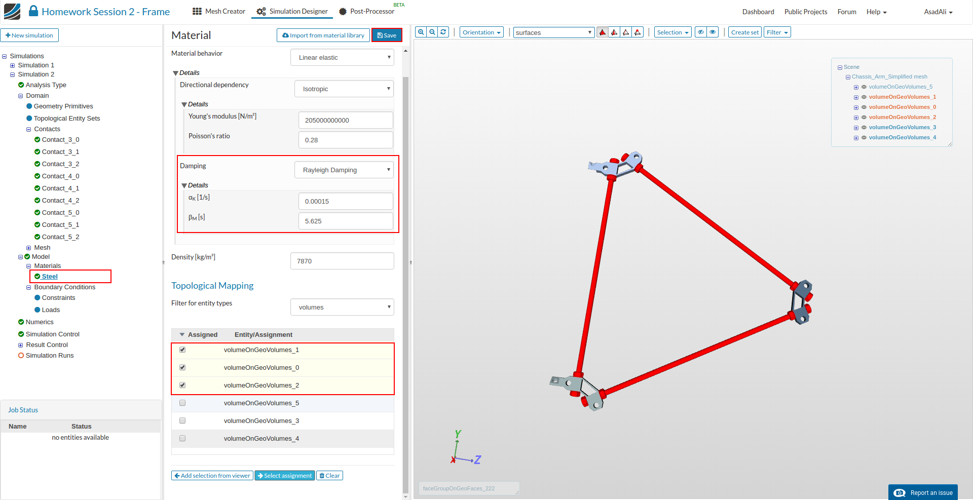
Please select steel from the list on the left side and save your selection by clicking the related button.
Change the damping propoties:
- Damping: Rayleigh Damping
- αK: 0.00015
- βM: 5.625
Now assign the material to the rods (volumeOnGeoVolumes_0, volumeOnGeoVolumes_1, volumeOnGeoVolumes_2).
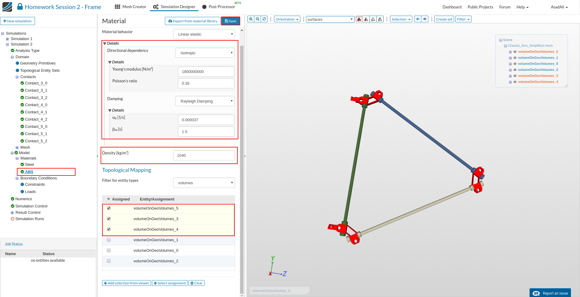
Please add a new material with following settings. Instead of using the library we have to define the material manually:
ABS Thermoplastics
- Name: ABS
- Young’s Modul: 1800000000
- Poisson’s ratio: 0.35
- Damping: Rayleigh Damping
- αK: 0.000037
- βM: 1.5
- Densiy: 1040
And assign it to the connectors (volumeOnGeoVolumes_3, volumeOnGeoVolumes_4, volumeOnGeoVolumes_5)
Please add, now, the same two constraint boundary conditions, which we used for the previous simulation.
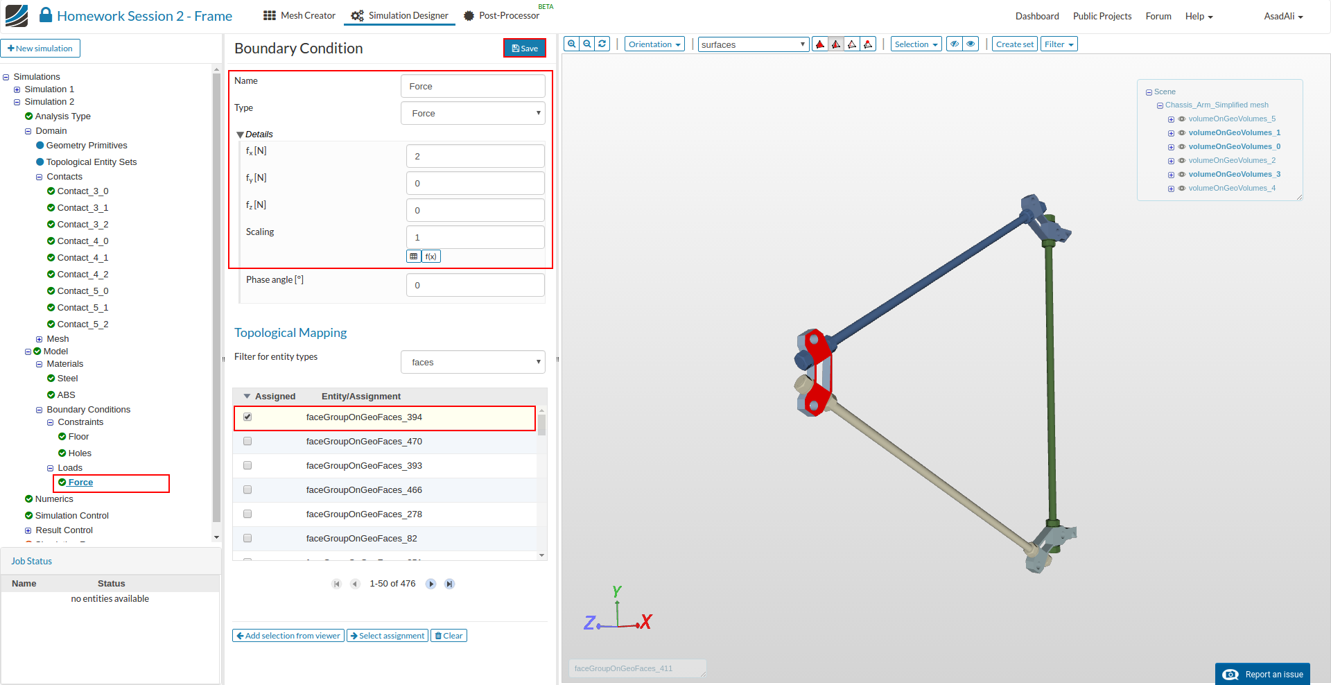
Next add a *Load boundary condition:
- Name: Lift
- Type: Force
- fx: 2
- fy: 0
- fz: 0
- Scaling: 1
Finally, assign the boundary condition to the faceGroupOnGeoFaces_394 (volumeOnGeoVolumes_3)
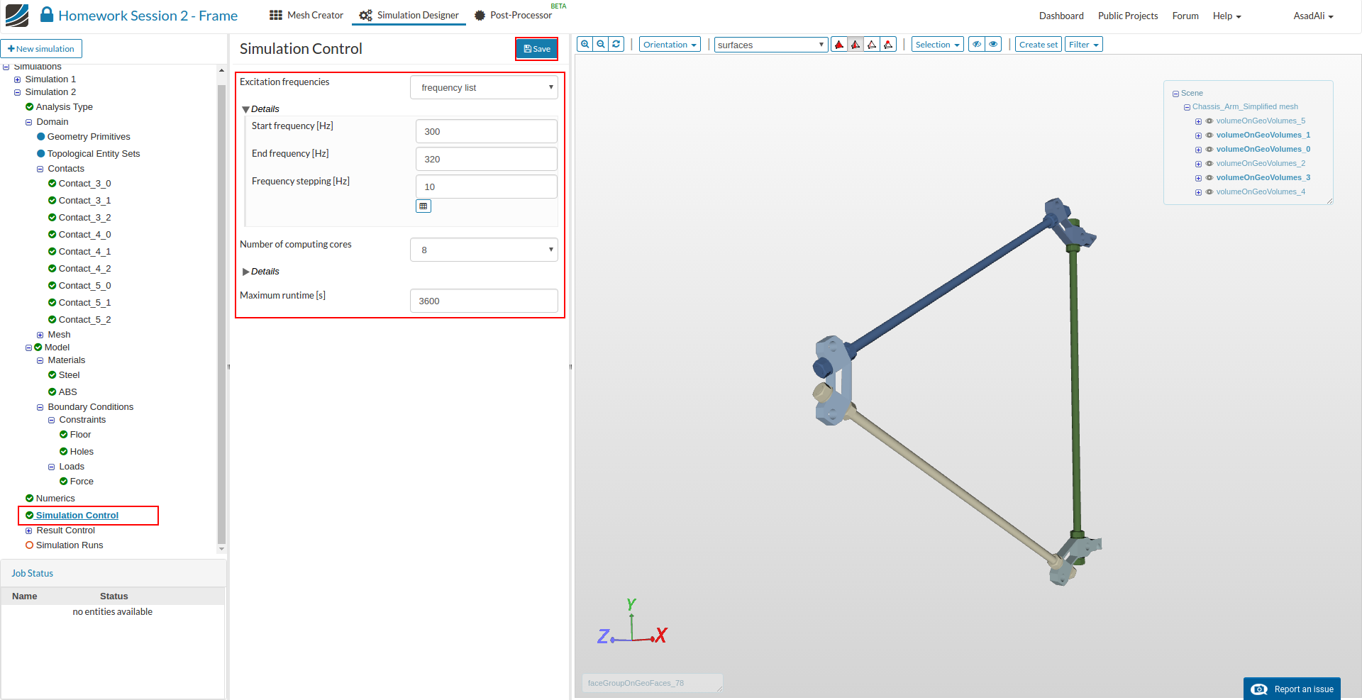
Click on the Simulation Control item in the project tree to specify the last details of your simulation.
Excitation frequencies: frequency list
Start frequency: 300
End frequency: 320
Frequency stepping: 10
Number of computing cores 8
Maximum runtime: 3600
Please choose the frequency band you want to investiagte yourself (based on the results of the frequency analysis. At least you should create four different runs with different frequency bands
Finally create a new run and start it.